From Noise to Insight: How Filtering Improves 3D Data Visualization
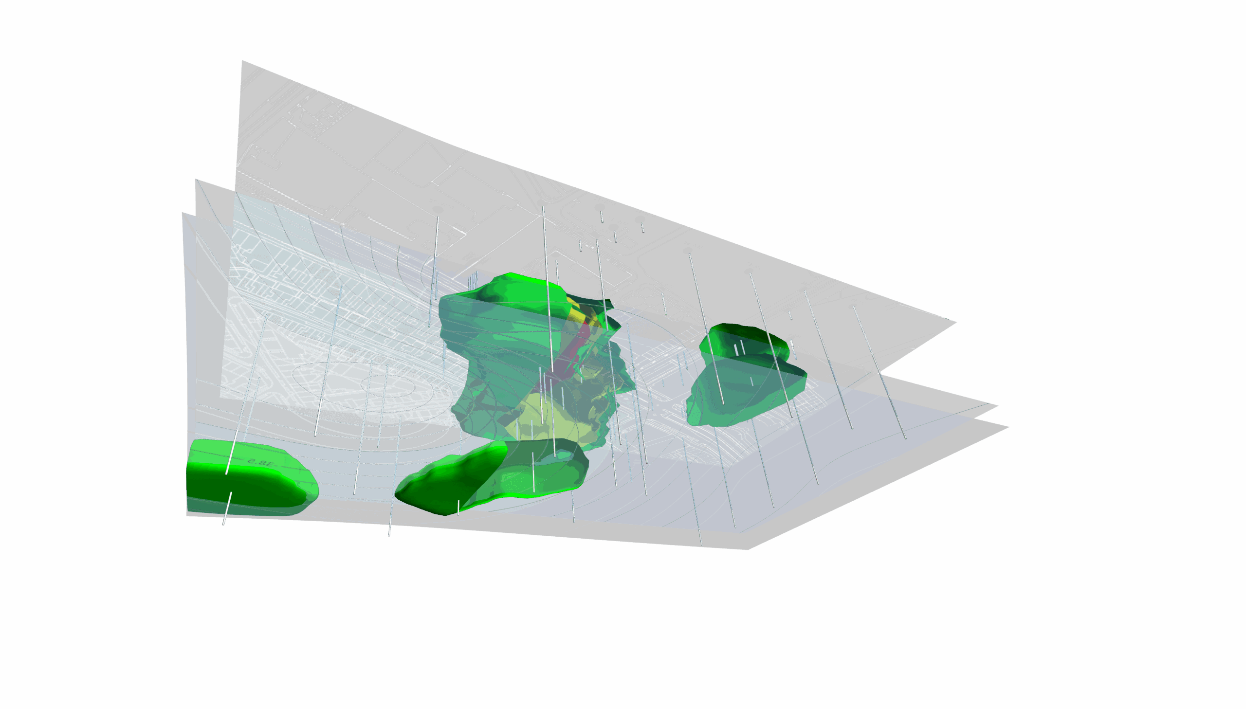
Visualizing data in 3D is transforming how you explore and communicate complex subsurface conditions. With volume renders, isosurfaces, image slices, and other 3D visualizations, you can model contaminant plumes, ore bodies, groundwater systems, and geological features that are difficult to understand from flat maps alone.
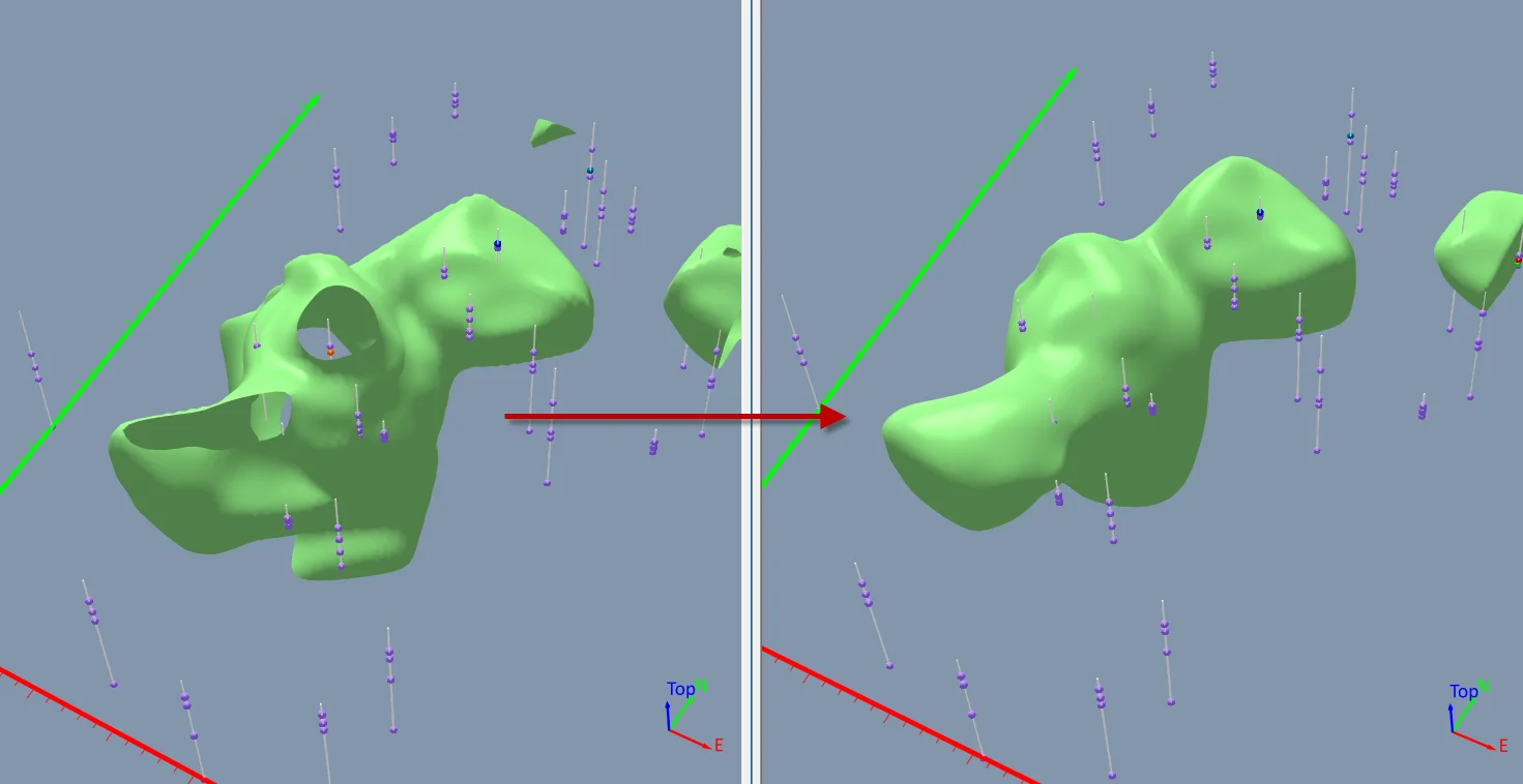
But even the best 3D visuals depend on the quality of the underlying grid. Raw 3D grids can contain noise, acquisition artifacts, or areas of missing data (NoData) that distract from the patterns you’re trying to understand. Left unaddressed, these imperfections can obscure important subsurface features, complicate interpretation, and reduce the clarity of your 3D data visualization.
Fortunately, refining a grid doesn’t mean starting your workflow from scratch. With the right 3D grid filters, you can create clearer, more informative outputs—all without modifying your original source data.
How 3D Grid Filtering Works
Before choosing a filter, it helps to understand how 3D grid filtering actually works. For this discussion, we’ll focus specifically on the 3D grid filters available in Surfer, since implementation can vary between software platforms.
The first concept to understand is that filtering in Surfer is non-destructive. Rather than modifying your original 3D grid, filters only change how the data is rendered in a visualization. That means you can experiment with different filters, compare results, and refine your presentation without worrying about altering your source dataset.
When you know the original data remains untouched, the next question becomes: how do the filters decide what changes to make? That answer lies in a handful of settings that dictate how each filter operates. While every filter serves a different purpose, they all rely on the same core controls. Understanding those controls will make it easier to choose the right filter and apply it effectively. Below are the main settings you’ll encounter in Surfer.
Kernel size
A filter doesn’t evaluate just one grid node at a time. Instead, it examines a surrounding neighborhood—called a kernel—before calculating the output value.
In Surfer, kernel sizes are defined using odd integers ranging strictly from 3 to 9. The center of that kernel is the node being evaluated, while the surrounding nodes provide the context the filter uses.
Depending on your chosen orientation, the kernel adjusts its dimensions accordingly:
- In 3D Volumetric Mode: The kernel acts as a cubic array in 3D space, ranging from 3 x 3 x 3 up to 9 x 9 x 9.
- In 2D Planar Mode (XY, XZ, or YZ): The filter operates slice-by-slice using a 2D matrix (such as 3 x 3 or 5 x 5).
In general, smaller kernels (like 3) preserve more local detail, while larger kernels (like 9) produce broader smoothing or more pronounced filtering effects because they incorporate information from a larger neighborhood.
Orientation
Not every filter has to operate on an entire 3D volume.
Depending on your objective, you can apply filters in different orientations. You can filter within a single XY, XZ, or YZ plane when refining individual slices, or apply a true 3D volumetric filter that evaluates neighboring nodes across all three dimensions simultaneously.
Choosing the appropriate orientation depends on whether you’re refining a single cross-section or the entire 3D dataset.
Edge handling
Filtering becomes more complicated along the edges of a grid because neighboring cells don’t exist beyond the dataset boundary.
To address this, Surfer provides several edge-handling methods, including:
- Replicate — Extends the outermost values beyond the grid boundary.
- Mirror — Reflects values across the edge to continue the surrounding pattern.
- Ignore — Uses only the neighboring cells that exist within the dataset.
- Cyclic Wrap — Wraps values from the opposite side of the grid, treating the dataset as though it repeats.
The option you choose determines how the filter behaves near the edges of the 3D data visualization and can influence the appearance of boundary regions.
NoData handling
Many geological models contain areas where data simply doesn’t exist. Rather than assigning estimated values everywhere, those locations are stored as NoData.
Surfer gives you several ways to control how filters interact with those blank regions, including:
- Leave Alone — Preserves the original NoData regions.
- Expanded — Grows NoData regions when neighboring cells are also blank.
- Ignore — Interpolates across nearby NoData values during filtering, which can reduce the size of blank regions.
Selecting the appropriate option depends on whether preserving data boundaries or creating a smoother visualization is more important for your analysis.
Note: When filtering isosurfaces or contour slices, remember that filters can change the range of values within the grid. As a result, existing isosurface or contour levels may temporarily disappear until the 3D data visualization automatically adjusts to the new data range.
Choosing the Right 3D Grid Filter for Your Goal
Now that we’ve covered how 3D grid filters work, the next thing to consider is simple: which one should you use? This answer depends entirely on what you’re trying to accomplish.
Some filters reduce noise, while others preserve sharp boundaries, highlight subtle geological features, or refine the final appearance of your visualization. Rather than searching for a single “best” filter, start by identifying the outcome you want your 3D data visualization to achieve. Below are a few realistic goals and which filters can help accomplish them.
1. Reduce noise and reveal regional trends
When a dataset contains noise, subtle geological patterns can become difficult to recognize. In these situations, smoothing filters help reduce unwanted variation so larger trends become easier to interpret.
Some of the most common smoothing filters include:
- Average (Rectangular) — Applies a uniform moving average across a rectangular neighborhood, giving every surrounding node equal influence.
- Average (Spherical) — Similar to the rectangular average but uses a spherical neighborhood to minimize corner bias.
- Distance — Calculates a distance-weighted average that gives greater influence to nearby nodes.
- Distance (Inverse) — Uses inverse distance weighting to further emphasize the closest neighboring values.
- Distance ‘Inf Norm’ — Applies distance-weighted averaging that results in concentric shoebox iso-weights.
- Gauss — Applies a bell-shaped Gaussian weighting that gently smooths noise while preserving the overall character of the dataset, making it a popular choice for publication-quality 3D data visualizations.
These filters are especially useful when working with continuous geophysical grids, seismic attribute volumes, or noisy bathymetric datasets, where the goal is to reveal broader regional patterns rather than emphasize small local variations.
2. Preserve boundaries while cleaning up noise
Sometimes reducing noise isn’t enough. You also need to preserve the sharp boundaries that define faults, ore bodies, contaminant plumes, or other important geological features.
Filters designed for structural enhancement include:
- Median — Replaces each node with the median value within its neighborhood, reducing isolated noise while preserving sharp boundaries.
- Maximum (Dilation) — Expands higher-value regions, making connected features easier to recognize.
- Minimum (Erosion) — Shrinks feature boundaries to remove isolated noise and better define core regions.
These filters work particularly well for ore body modeling, fault interpretation, and tracking localized contaminant concentrations, where preserving geological boundaries is just as important as reducing background noise.
3. Highlight hidden features and structural changes
Some filters are designed to help reveal features that might otherwise remain hidden.
Edge detection and feature extraction filters include:
- Prewitt, Sobel Max, and Sobel Norm — Compute directional derivatives across neighboring nodes to emphasize fractures, faults, and sharp structural boundaries.
- Laplacian Edge Detect — Applies a localized convolution kernel to detect rapid rate-of-change boundaries and outline structural edges.
- Unsharp Mask — Sharpens subtle visual features by calculating the difference between the original grid and a blurred version, helping fine geological structures stand out.
- Threshold Crossing — Converts voxels to binary indicators based on whether values cross a specified numerical threshold, making it ideal for mapping regulatory limits or concentration boundaries.
- Zero Crossing — Identifies exact locations where grid values transition from positive to negative to trace polarity changes and structural baselines. (Note: If your entire grid consists of single-sign values with no zero transitions, this filter will output all zeroes, which may cause contour slices or isosurfaces to disappear.)
These filters are particularly valuable for structural geological mapping, fault tracing, and identifying areas where measurements cross important geological or regulatory thresholds.
4. Fine-tune the final 3D data visualization
Not every filter is intended to reveal new geological insights. Sometimes the goal is simply to improve how the data is presented.
Filters for 3D data visualization refinement include:
- Bounding — Limits extremely high or low values to user-defined upper and lower bounds, reducing the visual impact of extreme outliers.
- Brightness, Contrast, and Gamma Correction — Adjust the appearance of the rendered visualization to improve understanding and emphasize important features.
These tools are especially useful when preparing figures for reports, presentations, and stakeholder communication, where a clearer 3D data visualization can make complex subsurface information much easier to understand.
Pro Tip: The Same Filter Can Improve Different Types of 3D Visuals
One of the advantages of filtering in Surfer is that the same filter can often improve several different types of 3D data visualizations. Depending on your workflow, you might:
- Apply a Gaussian or Median filter to create smoother volume renders and block renders.
- Use 2D planar filtering to clean up image slices or contour slices along specific cross-sections.
- Combine smoothing filters with appropriate NoData handling to create cleaner isosurfaces around concentration zones.
If you’re applying the same settings across multiple layers, Surfer also equips you to quickly copy and paste filter formatting so you can maintain consistent visualization settings throughout an entire project.
Turn Your Grid Into a Clearer 3D Data Visualization
The goal of 3D grid filtering isn’t to change what your data says but to remove the visual distractions that make the insights harder to see. By refining how your data is presented without modifying the original grid, you can create 3D data visualizations that are easier to interpret and communicate with confidence.
Whether you’re preparing figures for analysis, reports, or stakeholder presentations, Surfer’s non-destructive 3D grid filters help transform raw grids into clear, defensible visualizations that support better decision-making.
Which 3D filtering techniques are you most excited to use? Share your thoughts in the comments below!
Recent Articles
- Sep 23, 2026|Gabbie Rhodes|8 min
The best 3D data visualizations depend on the quality of your underlying grid. To achieve a great result, sometimes you need to use 3D grid filters.
- Sep 23, 2026|Gabbie Rhodes|11 min
When you're working with complex data, you need to communicate clearly. Graphs can help, especially when you follow design best practices.
- Sep 16, 2026|Gabbie Rhodes|7 min
The latest Surfer release delivers smarter 3D modeling, cleaner maps, and faster workflows. Unlock these benefits by discovering the top features.
- Sep 9, 2026|Gabbie Rhodes|4 min
Explore how Submara Survey bridged the gap between terrestrial elevation data and underwater bathymetry to guide costal development in Norway.