Visualizing Technical Data (Part 4): How to Visualize Climate Change Data Across Location and Time

Writer

Thought Leader

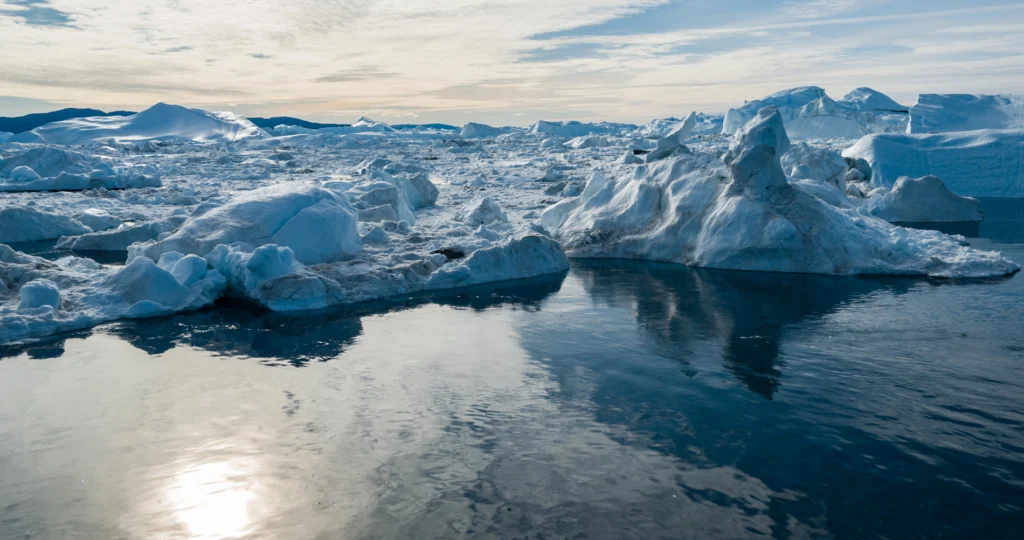
Climate change data rarely tells its full story from a single point in place or time. You may be working with temperature measurements, precipitation records, extreme-event metrics, or decades of observations from weather and climate stations. The challenge is making sense of where changes in temperature, precipitation, and other climate-related variables are occurring—and how those measurements are changing over time.

That’s where using both maps and graphs becomes valuable. Rather than relying on one type of visualization to capture every dimension of your data, showcasing climate change data often requires looking at the same story from both a spatial and temporal perspective.

In Part 4 of our Visualizing Technical Data blog series, we’ll explore how maps and graphs can help you examine climate change data across locations and time, and how connecting the two uncovers patterns that may be difficult to recognize from either perspective alone.

Why Is Climate Change Data Difficult to Visualize?

Before looking at how maps and graphs can help, it’s useful to understand why visualizing climate change data can be particularly challenging. Simply put, climate datasets are often multidimensional, requiring you to consider not only multiple variables, but also where and when those measurements were collected.

Depending on what you’re investigating, you may be working with data from numerous monitoring stations across different elevations and geographic settings. Those measurements may vary seasonally and annually, reveal longer-term trends, or include unusual and extreme observations. Even the same variable, such as temperature or precipitation, can show very different patterns depending on where and when it was measured.

That means your analysis may need to answer several different questions:

Where was the data collected?
How do measurements vary geographically?
How have measurements changed over time?
Do different locations show similar or different trends?
Are apparent anomalies isolated observations or part of a broader pattern?

Trying to answer all of these questions with one type of visualization can leave important context out of the picture. Fortunately, maps and graphs provide complementary views of the same climate data, equipping you to examine its spatial and temporal dimensions separately and then connect what you learn from both.

Use Maps to Understand Where Climate Conditions Occur

Let’s start with what maps bring to your analysis: geospatial context. Before comparing how climate measurements have changed over months, years, or decades, it helps to understand where those measurements originated and what’s around them.

Maps can provide that context by connecting climate measurements to the geography and terrain of your project area. They can also showcase monitoring locations with other spatial data so you can investigate how climate-related measurements vary from place to place. Let’s take a closer look at what all of this means.

Put monitoring locations into geographic context

Instead of comparing measurements from multiple stations immediately, you may need to ask: Where were those measurements collected, and how do those locations differ geographically?

Station-location point maps and base maps layered together can show weather or climate stations alongside relevant features such as:

regional boundaries and latitude
coastlines and marine proximity
rivers, lakes, and watersheds
urban centers (highlighting potential heat-island effects)
land cover and vegetation type

Seeing this information together can help you understand how monitoring stations are distributed across your project area and which surrounding features may be useful to consider when interpreting differences among locations.

For instance, plotting inland stations alongside coastal stations on a regional map makes it immediately clear how marine proximity buffers daily temperature swings, giving you essential geographic context before you start comparing their long-term trend lines.

Understand the role of elevation and terrain

Geographic location isn’t the only geospatial context that could matter. You may also need to ask: How do the elevations and surrounding terrain of monitoring locations differ?

Contour maps, color-relief maps, shaded-relief maps, and 3D terrain visualizations can help you examine elevation differences, mountain ranges, valleys, slopes, and the position of monitoring stations relative to those features. This context can be particularly useful when comparing climate measurements collected at locations with substantially different elevations or topographic settings.

Perhaps you’re comparing temperature records from several weather stations. Overlaying those stations on an elevation contour or color-relief map could reveal that they sit at considerably different elevations, giving you important context to consider as you investigate differences in their temperature records.

See how climate variables vary across a region

Another important question you may find yourself asking is: How does a climate-related variable change across the broader project area?

Depending on the available dataset, you might map temperature, precipitation, or another climate-related measurement using contour maps, color-relief maps, classified maps, or point maps symbolized by measurement. These visualizations can help reveal comparatively high or low values, spatial gradients, regional differences, and broader geographic patterns.

However, when creating a continuous surface from measurements collected at individual stations, it’s important to remember that values between measured locations are estimates produced through interpolation. The resulting surface depends on factors such as the available station network and the interpolation method used, so your visual should be interpreted accordingly.

For example, if you create a continuous surface map of regional rainfall, a sparse network of mountain weather stations might cause an interpolated model to smooth over localized microclimates or rain shadows. Recognizing that the map shows estimated gradients between stations will help you evaluate where additional monitoring points—or secondary data like satellite imagery—are needed to refine the surface.

Use Graphs to Understand How Climate Conditions Change Over Time

Maps can establish the geospatial context behind climate measurements, but that’s only one dimension of the story. Climate datasets often contain measurements collected repeatedly over years or decades, which raises another important question: How have those measurements changed over time?

That’s where graphs become particularly valuable for visualizing climate change data. They can help you examine long-term trends, compare records from multiple monitoring locations, and place variability and unusual observations within the context of a longer record. To highlight these capabilities more clearly, here’s a deeper look at how graphs help your analysis.

Track long-term changes in climate variables

When you have measurements collected repeatedly over an extended period, you might want to know: How has a particular climate variable changed across the available record?

Time-series and line graphs can help you examine temperature, precipitation, and other repeatedly measured climate variables across months, years, or decades. Depending on the dataset, these graphs can reveal long-term increases or decreases, shorter-term fluctuations, periods of relatively rapid change, and differences across portions of the observational record.

For instance, you could graph the annual average temperature from a particular weather station over several decades. While the measurements may fluctuate from year to year, viewing the complete record can help you determine whether a longer-term trend is also present.

Compare climate trends across locations

Once you’ve used maps to understand where monitoring stations are located, you can ask another question: Do measurements from different locations show similar or different patterns over time?

Multi-series time plots and comparative line graphs can place records from several monitoring locations along the same timeline. This makes it easier to examine similarities and differences in trends, identify periods when records diverge or converge, and compare patterns of change among locations.

Perhaps you’ve mapped several weather stations across varying terrain and now want to compare their multi-decade temperature records. Multi-series graphs make it easy to see if a high-elevation station and a valley station share the exact same warming trajectory, even if their baseline temperatures sit 5°C apart due to elevation differences.

Put variability and unusual observations into context

Long-term trends aren’t the only thing worth investigating. Climate measurements naturally fluctuate, which means you may also need to wonder: What’s typical for the dataset, how much does it vary, and are any observations unusual within that broader context?

Box plots and histograms can help you investigate questions like:

What values or ranges are most common?
How much variability is present within the data?
How does the distribution differ among locations or time periods?
Are there potential outliers or unusual observations worth investigating?

For example, you could use box plots to compare temperature measurements from different time periods or monitoring stations. Rather than focusing on individual high or low observations, you could examine how the overall distributions compare, including differences in typical values, spread, and potential outliers.

Connect Maps and Graphs to See the Full Climate Story

Maps and graphs each reveal a different dimension of climate data, but the real analytical value comes from moving between the two. A pattern you notice on a map may lead you to investigate how measurements have changed over time, while something unusual in a graph may send you back to the map for geographic context. To put this into greater perspective, here’s an example.

Say you’re analyzing temperature data collected from several weather stations across a region. You could start by mapping the monitoring network to understand where each station is located. Adding elevation, terrain, coastlines, water bodies, or other relevant geographic features could then provide additional context about the physical settings surrounding those stations.

Next, you might map average temperature across the region for a defined period to examine broader spatial patterns. If certain locations stand out, you could select stations in those areas and create time-series graphs of their temperature records. Now, instead of seeing only how temperatures differ spatially, you can investigate how measurements at those locations have changed across years or decades.

Comparing those graphs may also reveal another layer of the story. Perhaps two stations have noticeably different absolute temperatures but show a similar long-term direction of change. Returning to your map could reveal that the stations sit at substantially different elevations, providing useful context for interpreting why their temperature measurements differ even though their longer-term patterns may be similar.

The analysis could also work in the opposite direction. A time-series graph might reveal that one station’s record behaves differently from those of nearby stations. That finding could prompt you to return to the map and examine whether the station’s elevation, location, or surrounding geographic setting differs in a way that’s relevant to your interpretation.

This back-and-forth is where combining maps and graphs becomes especially valuable for visualizing climate change data. Maps give temporal patterns a geographic setting, while graphs show how measurements from those locations behave through time. By connecting the two, you can investigate climate data from multiple perspectives and build a more complete picture than either visualization could provide on its own.

Connect Location With Change Over Time

Climate change data has a lot of dimensions to consider at once. Geography, time, variability, and multiple measurements can all play a role in the patterns you’re trying to understand. That’s why effective climate change data visualization often requires more than one view of the data.

Maps can show where measurements originated and how climate-related variables vary across an area, while graphs can reveal how those measurements change, fluctuate, and compare over time. Neither perspective necessarily tells the complete story on its own. Connecting the two can help you investigate patterns more thoroughly while giving stakeholders the geographic and temporal context they need to understand what those patterns mean.

But there’s more to explore when it comes to the benefits of using both maps and graphs. In the final post of our Visualizing Technical Data blog series, we’re turning our attention to earthquake data and exploring how different visual perspectives can help you better understand seismic activity and the patterns hidden within the information.

Until then, how do you combine spatial and temporal visualizations when working with climate change data? Leave a comment below and share the map-and-graph combinations that have been most useful in your work.