Visualizing Technical Data (Part 5): How to Showcase Data on Earthquakes to Highlight Key Insights


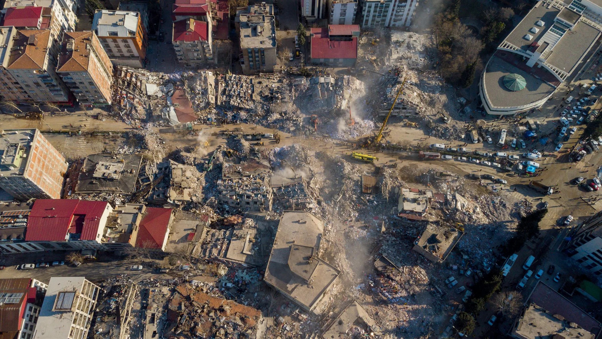
An earthquake may appear as a single point on a map, but there’s much more behind that dot. Where did the earthquake occur? How strong was it? How deep was it? How often are similar events happening? And what patterns emerge when you look across multiple events over time?
Answering those questions means working with data on earthquakes that can span location, magnitude, depth, frequency, and time. But because those variables tell different parts of the story, trying to understand them through a single type of visualization can leave important insights out of view. That’s why you need to rely on both maps and graphs.
In the fifth and final installment of our Visualizing Technical Data blog series, we’re exploring how both maps and graphs can help you investigate earthquake data from multiple angles, uncover deeper insights, and communicate findings more effectively.
Why Data on Earthquakes Requires Various Types of Visuals
First things first: let’s dive deeper into why multiple types of visualizations are necessary when showing data on earthquakes. In a nutshell, this technical data can contain several pieces of information that answer key questions. A dataset, for example, may include event locations, magnitudes, depths, frequency, and dates and times.
With that information, you may want to know:
- Where are the earthquakes occurring?
- How do their locations relate to faults, terrain, or defined hazard zones?
- How strong are the recorded earthquakes?
- How frequently are earthquakes of different magnitudes occurring?
- What patterns become apparent when you consider the spatial and analytical perspective of the data together?
No single visualization will answer all of those questions equally well. A map, for instance, makes it easy to spot clusters of seismic activity and see where events occur relative to surrounding features. But it may be harder to use that same visual to understand the overall frequency or distribution of earthquake magnitudes. A graph, of course, could make those patterns easier to examine, but without a map, you’d lose the geographic context behind the measurements.
That’s why utilizing both maps and graphs lead to a more complete view of your earthquake data. Maps will help you investigate the spatial side of seismic activity, while graphs will empower you to dig deeper into the magnitude, frequency, and other patterns behind those events.
Use Maps to Understand Where Earthquakes Occur
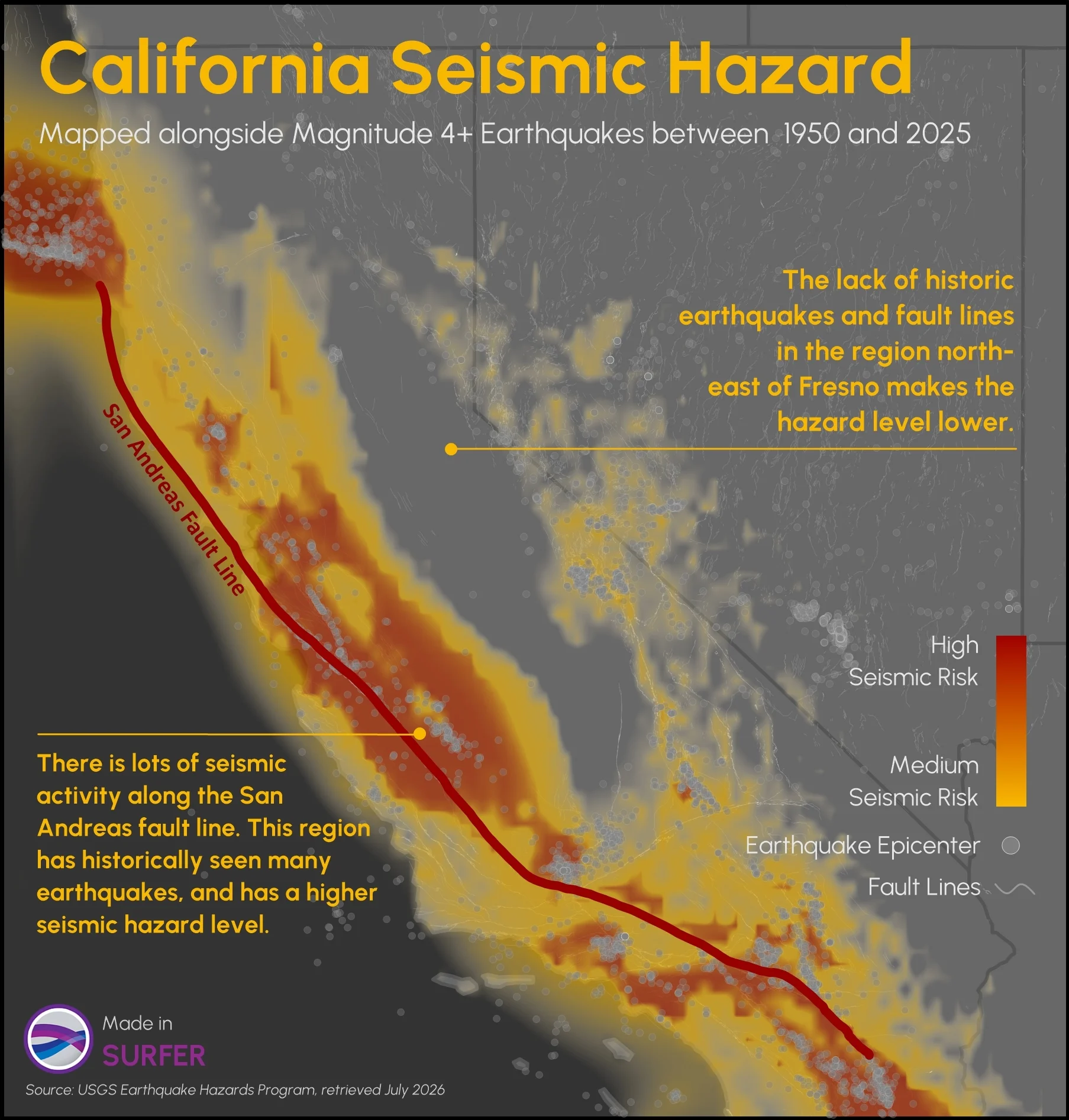
Now, let’s walk through the specific benefits maps play in visualizing data on earthquakes. When it comes to seismic activity, maps can establish where those events occurred and place them within a broader geographic setting. If you combine earthquake locations with faults, terrain, hazard zones, and other spatial information, you can also start exploring not just where earthquakes are happening, but what spatial patterns and relationships may exist around them. Here’s more insight on what that looks like practically.
Put earthquake events into geographic context
Perhaps you want to ask: Where are earthquakes occurring, and what’s around those locations?
A post map can plot individual earthquake events across your study area, giving you a straightforward view of where seismic activity has been recorded. From there, you can add base maps containing fault lines, hazard-zone boundaries, coastlines, administrative boundaries, and other geographic features relevant to your analysis.
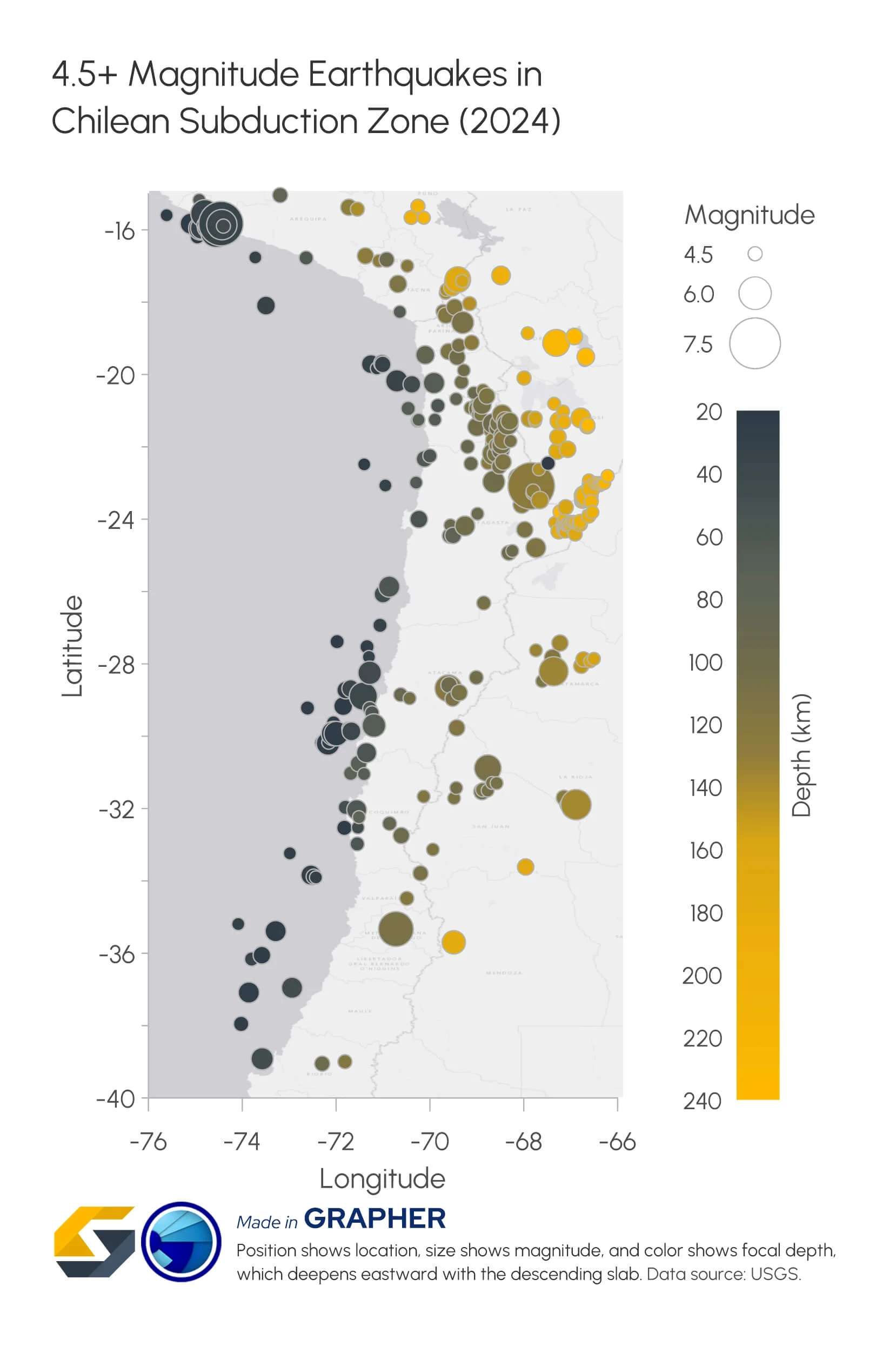
You can also vary the symbols used for individual events based on information in your dataset. If you have magnitude data, for example, changing symbol size based on magnitude can help you distinguish stronger and weaker events while still seeing where each one occurred.
Examine earthquake depth alongside location
Mapping earthquake epicenters across the surface is only part of the story. Because seismic events originate deep underground, it raises another critical spatial question: How is that seismic activity distributed vertically throughout the subsurface?
A 3D post map can use the X, Y, and depth values in your dataset to display earthquake hypocenters in three dimensions. Rather than representing every event on the same flat plane, you can investigate how seismic activity is distributed both horizontally and vertically.
When elevation data is available, you can also drape a color-relief terrain map across the land surface to provide immediate top-down context over your subsurface hypocenters. Additionally, symbol properties can represent another variable, such as magnitude, equipping you to evaluate location, depth, and event strength simultaneously within a single 3D visualization.
For example, plotting scaled hypocenter spheres beneath a 3D terrain surface equips you to instantly see whether high-magnitude quakes are concentrated along a deep subduction fault or scattered near the surface. This can help you identify whether stronger events correlate with specific subsurface fault structures or remain isolated at shallow depths.
Identify broader spatial patterns in seismic activity
Once individual earthquake locations have context, you can zoom out and ask: Do the events form noticeable spatial patterns?
A post map can help you examine the overall distribution of recorded earthquakes and identify areas where events appear to cluster. If you want to distinguish between categories of events, a classed post map can group and symbolize earthquakes according to a variable such as magnitude or depth.
You can then combine those event locations with additional map layers to provide more context for the patterns you see. Contour or color-relief maps can represent elevation or another relevant continuous spatial variable, while base maps can add faults or hazard-zone boundaries.
For instance, you could create a classed post map that distinguishes earthquakes by magnitude range and overlay known fault lines using a base map layer. That combination would equip you to investigate not only where earthquakes are concentrated, but also whether stronger and weaker events show different spatial patterns in relation to those faults.
Use Graphs to Understand Earthquake Magnitude and Frequency
After you’ve explored where earthquakes are occurring, you can shift your attention to what the measurements behind those events reveal. That’s where graphs come into play. They pull variables such as magnitude, frequency, and time into focus. This can make it easier to compare recorded events and recognize statistical or temporal patterns that may be difficult to see from their locations on a map alone. To highlight these capabilities, here’s a closer look at how graphs support seismic analysis.
Understand how frequently earthquakes of different magnitudes occur
One question you may want to investigate is: How often are earthquakes occurring at different magnitudes?
A classed bar chart can help answer that question by grouping recorded earthquakes into magnitude ranges and displaying the number of events within each class. This will give you a clearer view of the overall distribution of earthquake magnitudes, including which ranges contain the most events and how frequently stronger earthquakes appear compared with weaker ones.
For example, grouping a regional earthquake dataset into magnitude bins—such as 2.0–2.9, 3.0–3.9, and 4.0+—in a classed bar chart immediately reveals whether your study area is experiencing hundreds of low-magnitude micro-tremors punctuated by rare major events, or if activity is concentrated in a narrower, moderate-intensity band.
Compare the magnitudes of recorded earthquakes
You may also want to ask: How severe are the earthquakes represented in the dataset? Graphs can make individual earthquake magnitudes easier to compare by temporarily separating those measurements from their geographic locations. This can help comparatively strong or weak events stand out from the rest of your dataset.
For example, plotting recorded events on a scatter plot can help you quickly isolate the top 5% largest events in a catalog spanning thousands of earthquakes. By setting visual threshold lines for key levels—such as magnitude 5.0+—you can instantly filter out routine background activity and highlight the specific high-impact events that warrant deeper structural risk analysis.
Investigate patterns over time
If your earthquake dataset includes timestamped records, another question becomes possible: How has recorded seismic activity evolved across your study window?
Time-series graphs make it easy to evaluate changes across the full duration of your dataset. Depending on what you plot, you can track fluctuations in event frequency, identify intervals of heightened activity, or observe how individual magnitudes shift month by month or year by year.
For example, plotting daily earthquake counts on a time-series line graph alongside a magnitude scatter plot across a multi-month period can clearly illustrate foreshock and aftershock sequences. The graph will equip you to pin down the precise timestamp of a mainshock event, observe the sharp spike in immediate aftershocks, and monitor how long it takes for regional seismic activity to return to baseline levels.
Connect Maps and Graphs to Reveal Deeper Insights From Your Data on Earthquakes
Mapping where earthquakes occur and graphing how they behave are powerful techniques on their own. But what does combining both perspectives actually look like in a real-world analysis?
Say you’re examining data on earthquakes recorded across a particular region. You could begin with a post map showing individual earthquake locations alongside fault lines, elevation, hazard-zone boundaries, or other relevant spatial information. As you create the map, perhaps you notice a cluster of seismic events in one part of the study area that warrants a closer look. Now you have a new question: What’s happening within that cluster?
This is where you can move from the map to your graphs. You could isolate the events within your area of interest and examine their magnitude and frequency. A classed bar chart, for example, could group those earthquakes by magnitude range and show how frequently events fall within each class. You may discover that most of the recorded events fall within a particular magnitude range, while a smaller number of stronger earthquakes stand out. Those findings can then give you a clear reason to revisit your spatial data.
You could map the stronger events and investigate where they occurred relative to the faults, terrain, or hazard zones you mapped earlier. Or, if a time-based graph reveals a period with a notable cluster of recorded events, you could map those earthquakes separately to see whether they were concentrated in the same area or spread across the region.
This back-and-forth is where maps and graphs are especially powerful. The map may reveal a spatial pattern that gives you a reason to investigate certain measurements. The graph may then uncover a pattern in those measurements that raises another question about location. Instead of treating each visualization as the final answer, you can let one insight guide the next stage of your analysis.
This complementary workflow also explains why different data visualization tools can play distinct roles in the same project. Surfer, for example, can support the spatial side of earthquake analysis by helping you map event locations and the surrounding area. Grapher, on the other hand, can support the analytical side by helping you visualize magnitude, frequency, and changes over time.
See the Full Story Behind Your Earthquake Data
Data on earthquakes can tell a comprehensive story. Location, magnitude, depth, frequency, changes over time, and relationships across events can all bring that story to life. However, as we’ve explored throughout this article, analyzing those different variables to see the full story often means looking at your data in more than one way.
That’s why maps and graphs are so valuable together. Maps reveal where seismic activity occurs and provide important spatial context, while graphs help you investigate magnitude, frequency, and changes over time. By connecting what you learn from both, you can build a more complete picture than either perspective can provide on its own.
How could you combine maps and graphs to get more from your earthquake data or another type of technical data? Let us know in the comments! We’d love to hear how you can put both perspectives to work.
Recent Articles
- Nov 18, 2026|Gabbie Rhodes|10 min
Maps and graphs can help you investigate data on earthquakes from multiple angles to uncover deeper insights and communicate more effectively.
- Nov 11, 2026|Gabbie Rhodes|8 min
Transforming complex datasets into clear, actionable visuals can help you understand tsunami behavior and risk, enhancing tsunami preparedness.
- Nov 4, 2026|Gabbie Rhodes|6 min
Discover how Alexey Shulgin, Chief Geophysicist at Submara Survey, used various visuals to inform a Norwegian city's dredging project.
- Oct 28, 2026|Gabbie Rhodes|8 min
For our 2026 All Hands Meeting, our team gathered in Colorado for a few days of workshops, customer conversations, and fun activities.